Pivots in tidyverse.
library(tidyverse)
library(lubridate)
library(zoo)
theme_set(theme_light(20))
Load some data
Daily air quality measurements in New York, May to September 1973. Temp: Maximum daily temperature in degrees Fahrenheit at La Guardia Airport.
df <- airquality %>%
        as_tibble() %>%
        select(day = Day, month = Month, temp = Temp, wind = Wind)
df
# A tibble: 153 x 4
     day month  temp  wind
   <int> <int> <int> <dbl>
 1     1     5    67   7.4
 2     2     5    72   8
 3     3     5    74  12.6
 4     4     5    62  11.5
 5     5     5    56  14.3
 6     6     5    66  14.9
 7     7     5    65   8.6
 8     8     5    59  13.8
 9     9     5    61  20.1
10    10     5    69   8.6
# … with 143 more rows
We add the year to create a date column. Let’s have a look on one variable.
df2 <- df %>% mutate(date = ymd(paste("1973",month,day,sep="-")))

ggplot(data = df2, mapping = aes(x = date, y = temp)) +
    geom_line()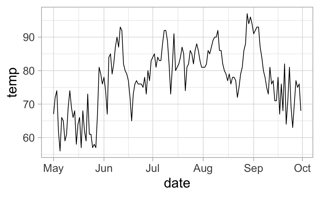
Now, adding the second variable.
ggplot(data = df2, mapping = aes(x = date)) +
    geom_line(aes(y = temp), colour = "blue") +
    geom_line(aes(y = wind), colour = "orange")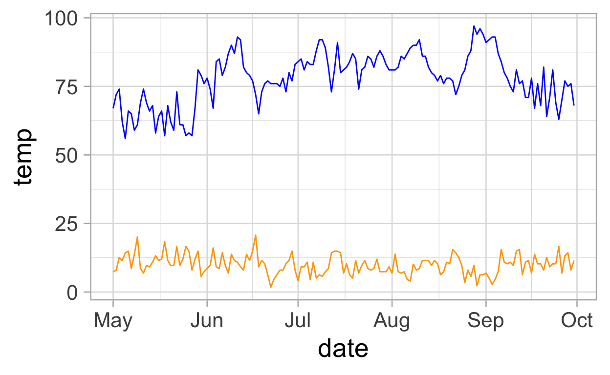
Problem
This js not nice and not a tidy way to map the data to aesthetics. We need a column with the information about the variable and a column with information about the value of the variable.
That means we have to transform the data from the wide format to a long format.
This is the Excel-like wide format (everybody is used to it):
df2
# A tibble: 153 x 5
     day month  temp  wind date
   <int> <int> <int> <dbl> <date>
 1     1     5    67   7.4 1973-05-01
 2     2     5    72   8   1973-05-02
 3     3     5    74  12.6 1973-05-03
 4     4     5    62  11.5 1973-05-04
 5     5     5    56  14.3 1973-05-05
 6     6     5    66  14.9 1973-05-06
 7     7     5    65   8.6 1973-05-07
 8     8     5    59  13.8 1973-05-08
 9     9     5    61  20.1 1973-05-09
10    10     5    69   8.6 1973-05-10
# … with 143 more rows
Solution: From wide to long data format
df_long <- df2 %>% pivot_longer(data = .,
            cols = c("temp", "wind"),
            names_to = "variable",
            values_to = "value")
df_long
# A tibble: 306 x 5
     day month date       variable value
   <int> <int> <date>     <chr>    <dbl>
 1     1     5 1973-05-01 temp      67
 2     1     5 1973-05-01 wind       7.4
 3     2     5 1973-05-02 temp      72
 4     2     5 1973-05-02 wind       8
 5     3     5 1973-05-03 temp      74
 6     3     5 1973-05-03 wind      12.6
 7     4     5 1973-05-04 temp      62
 8     4     5 1973-05-04 wind      11.5
 9     5     5 1973-05-05 temp      56
10     5     5 1973-05-05 wind      14.3
# … with 296 more rows
ggplot(data = df_long, aes(x = date, y = value)) +
    geom_line(aes(colour = variable))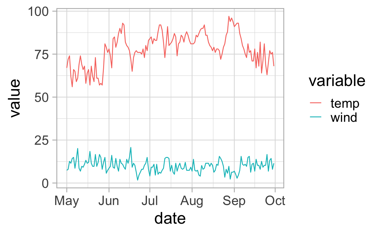
ggplot(data = df_long, aes(x = date, y = value)) +
    geom_line(aes(colour = variable))+
    facet_wrap(~variable, nrow = 1)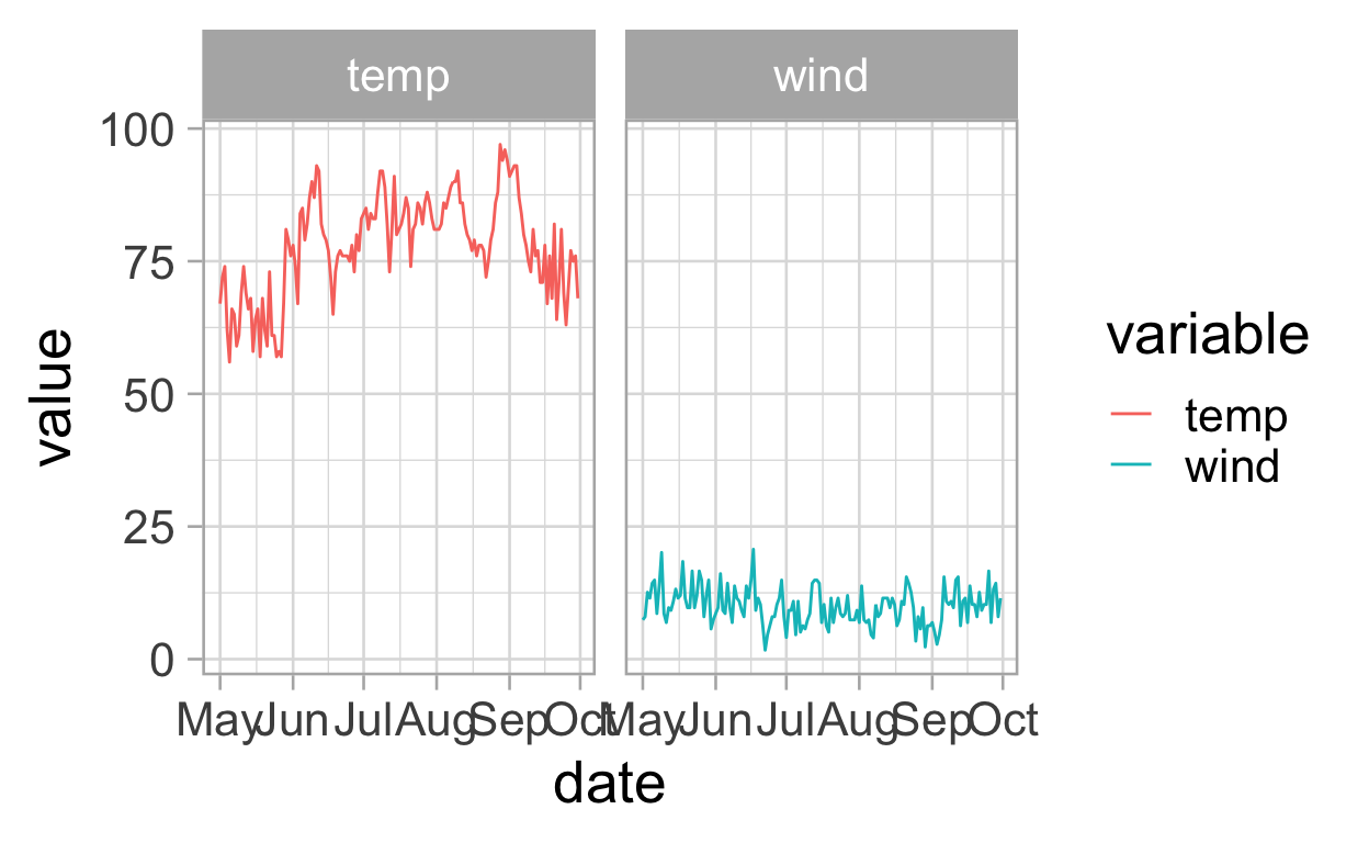
ggplot(data = df_long, aes(x = date, y = value)) +
    geom_line(aes(colour = variable))+
    facet_wrap(~variable, nrow = 2, scales = "free_y")+
    theme(panel.spacing = unit(50, "pt"))+ #more space between facets
    guides(colour = FALSE) # remove legend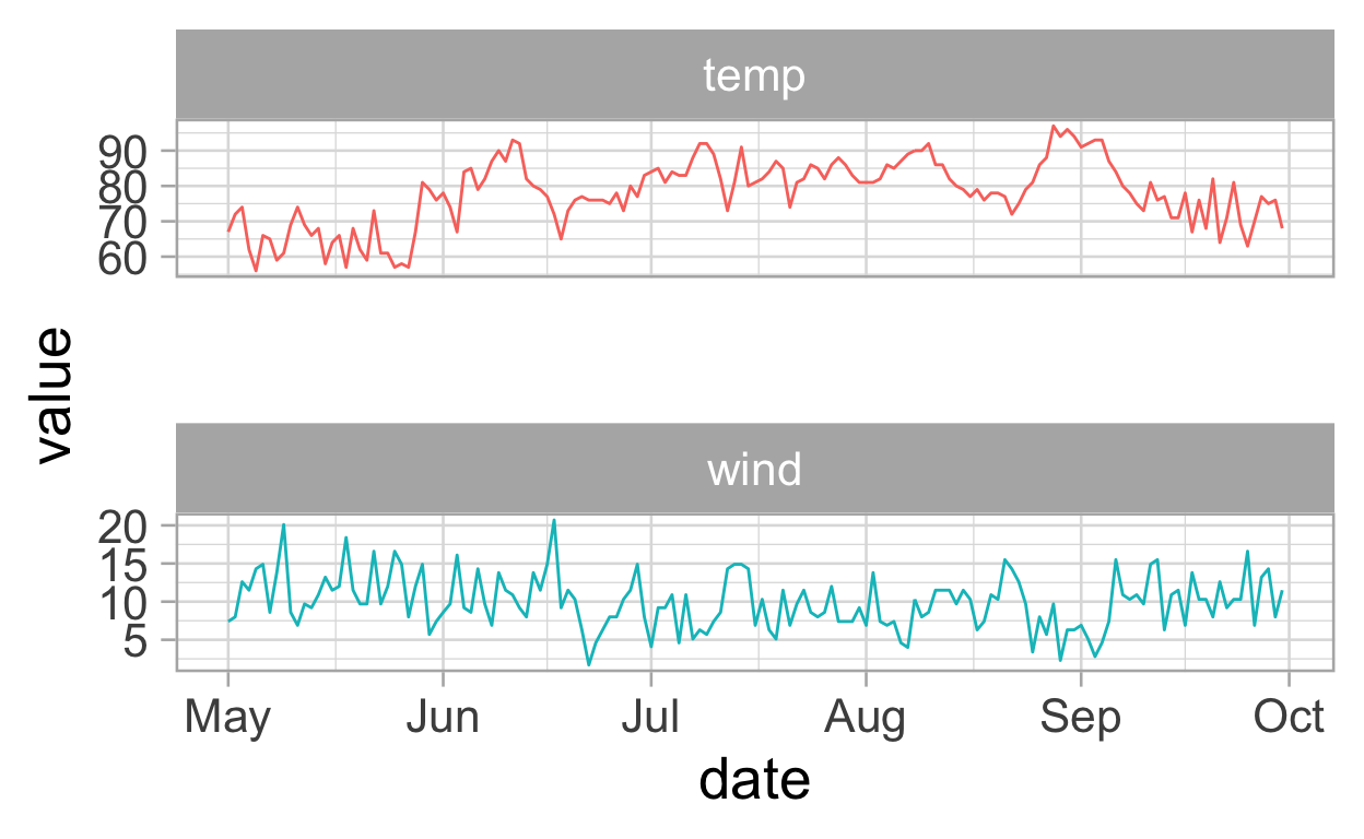
Long-data format gets more and more effective the more variables you have.
Now data analysis is also easier. For example you want to find the date in each month where are the maximum for each variable is measured.
df_long2 <- airquality %>%
        as_tibble() %>%
        pivot_longer(data = .,
                 cols = Ozone:Temp,
                 names_to = "var",
                 values_to = "value")
df_long2 %>%
    group_by(var, Month) %>%
    arrange(-value) %>%
    slice(1) %>%
    ungroup() %>%
    print()
# A tibble: 20 x 4
   Month   Day var     value
   <int> <int> <chr>   <dbl>
 1     5    30 Ozone   115
 2     6     9 Ozone    71
 3     7     1 Ozone   135
 4     8    25 Ozone   168
 5     9     1 Ozone    96
 6     5    16 Solar.R 334
 7     6    14 Solar.R 332
 8     7     6 Solar.R 314
 9     8    13 Solar.R 273
10     9    10 Solar.R 259
11     5    29 Temp     81
12     6    11 Temp     93
13     7     8 Temp     92
14     8    28 Temp     97
15     9     3 Temp     93
16     5     9 Wind     20.1
17     6    17 Wind     20.7
18     7    13 Wind     14.9
19     8    21 Wind     15.5
20     9    25 Wind     16.6
Instead of calculating the average for each variable you group_by() in the long tibble and summarise, done.
df_long2 %>%
    group_by(var) %>%
    summarise(avg = mean(value, na.rm = TRUE))
# A tibble: 4 x 2
  var        avg
  <chr>    <dbl>
1 Ozone    42.1
2 Solar.R 186.
3 Temp     77.9
4 Wind      9.96
From long to wide format
Backwards tranformation is also possible (back to wide format). Quote aorund the column names are not needed.
df_long2 %>% pivot_wider(data = .,
             names_from = var,
             values_from = value)
# A tibble: 153 x 6
   Month   Day Ozone Solar.R  Wind  Temp
   <int> <int> <dbl>   <dbl> <dbl> <dbl>
 1     5     1    41     190   7.4    67
 2     5     2    36     118   8      72
 3     5     3    12     149  12.6    74
 4     5     4    18     313  11.5    62
 5     5     5    NA      NA  14.3    56
 6     5     6    28      NA  14.9    66
 7     5     7    23     299   8.6    65
 8     5     8    19      99  13.8    59
 9     5     9     8      19  20.1    61
10     5    10    NA     194   8.6    69
# … with 143 more rows