Use sf() in data analysis
Load HOBO meta table
First, load a recent version of the HOBO meta table from the Google Sheet.
data <- read_csv("https://docs.google.com/spreadsheets/d/e/2PACX-1vS_m42YZdulaKJVngJZq51T5CEX36LlqkAnHzOoVmcZXpbHGZ_AofTknbrPGRfWS5PRQ9GygOgkEHdz/pub?output=csv", col_types  = cols())

meta <- data %>%
        as_tibble() %>%
        select(-name_anonym, -description)

meta %>% select(hobo_id, latitude, longitude)
# A tibble: 43 x 3
    hobo_id latitude longitude
      <dbl>    <dbl>     <dbl>
 1 10760706     48.0      7.83
 2 10347531     48.0      7.82
 3 10760815     48.0      7.86
 4 10350086     48.0      7.87
 5 10347319     48.0      7.84
 6 10350043     48.0      7.86
 7 10350009     48.0      7.84
 8 10350048     48.0      7.89
 9 10350051     48.0      7.81
10 10347346     48.0      7.81
# … with 33 more rows
Transform tibble to simple feature
With st_as_sf we define the geographic coordinates from the meta table as POINTS and set the coordinate reference system (here: 4326). Because there are HOBO locations outside the city of Freiburg, we use filter() to exclude those locations.
meta_sf <- st_as_sf(meta,
        coords = c("longitude", "latitude"),
            crs = 4326)

hobo_sf <- meta_sf  %>%
    st_transform(31467) %>%
    filter(region == "Freiburg")
Have a look into the Coordinate Reference Systems:
st_crs(hobo_sf)
Coordinate Reference System:
  EPSG: 31467
  proj4string: "+proj=tmerc +lat_0=0 +lon_0=9 +k=1 +x_0=3500000 +y_0=0 +ellps=bessel +towgs84=598.1,73.7,418.2,0.202,0.045,-2.455,6.7 +units=m +no_defs"
st_crs(meta_sf)
Coordinate Reference System:
  EPSG: 4326
  proj4string: "+proj=longlat +datum=WGS84 +no_defs"
Now load the Freiburg district shapefile stadtteile.shp available on github.
shpfile <- "~/Dropbox/IHF/Lehre/MSc/_Datenkurs/Datenkurs_2020/data/GIS/freiburg_districts_shp/stadtteile.shp"
frbg_districts <- st_read(shpfile)
Reading layer `stadtteile' from data source `/Users/modchembp/Dropbox/IHF/Lehre/MSc/_Datenkurs/Datenkurs_2020/data/GIS/freiburg_districts_shp/stadtteile.shp' using driver `ESRI Shapefile'
Simple feature collection with 28 features and 5 fields
geometry type:  POLYGON
dimension:      XY
bbox:           xmin: 3400154 ymin: 5307882 xmax: 3420277 ymax: 5326568
epsg (SRID):    31467
proj4string:    +proj=tmerc +lat_0=0 +lon_0=9 +k=1 +x_0=3500000 +y_0=0 +ellps=bessel +towgs84=598.1,73.7,418.2,0.202,0.045,-2.455,6.7 +units=m +no_defs
st_crs(frbg_districts)
Coordinate Reference System:
  EPSG: 31467
  proj4string: "+proj=tmerc +lat_0=0 +lon_0=9 +k=1 +x_0=3500000 +y_0=0 +ellps=bessel +towgs84=598.1,73.7,418.2,0.202,0.045,-2.455,6.7 +units=m +no_defs"
To join or plot different sf-objects later on be sure that the projection of both objects is the same.
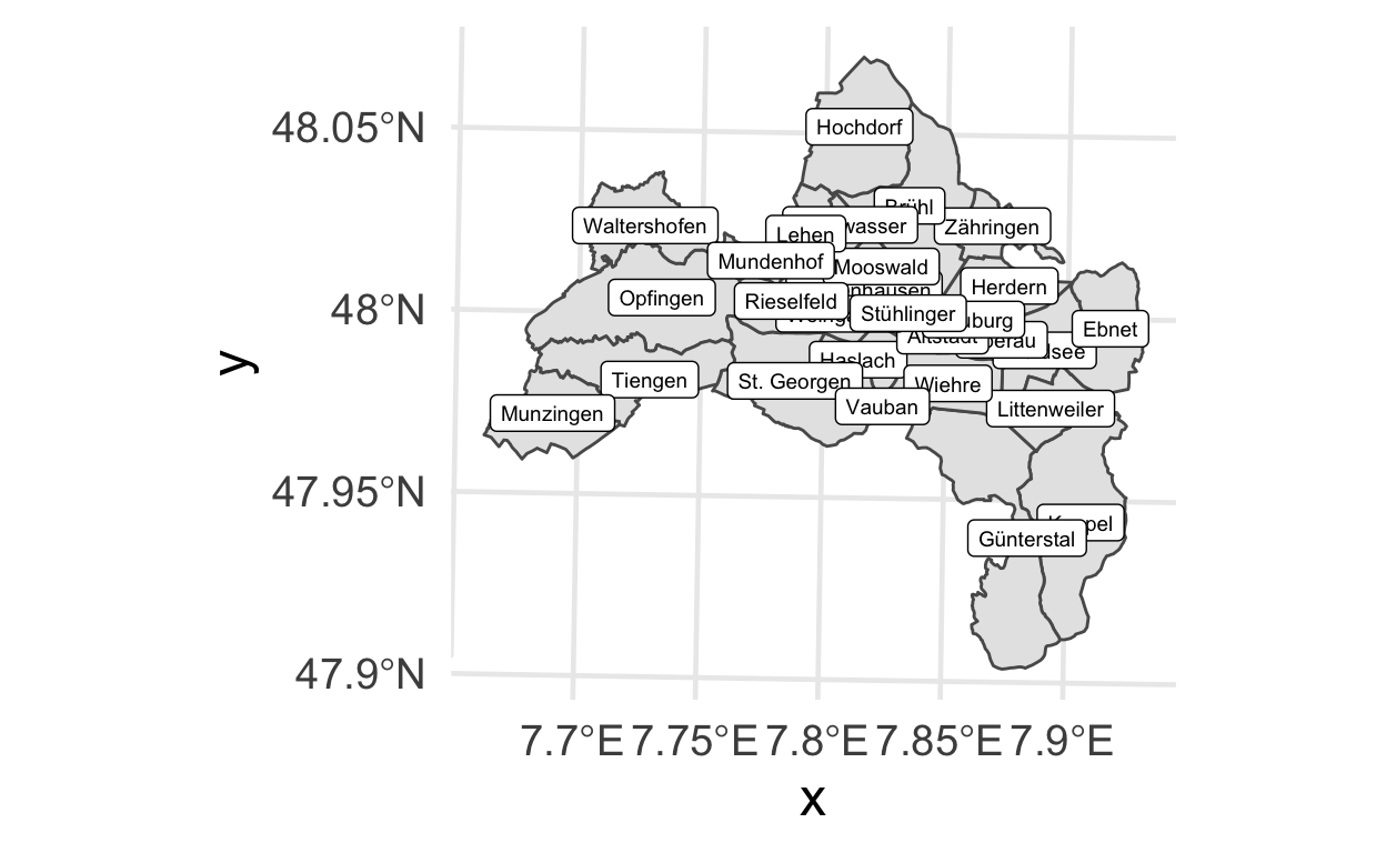
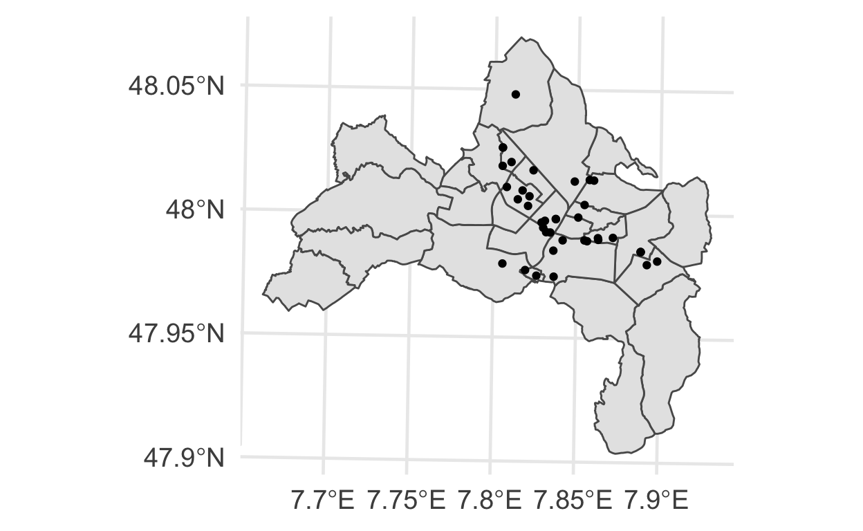
Plotting the districts in Freiburg with labels and then the locations of all HOBO stations.
ggplot(data = frbg_districts) +
    geom_sf() +
    geom_sf_label(aes(label = name), size = 2.5)+
    theme_minimal(18)
ggplot() +
    geom_sf(data = frbg_districts) +
    geom_sf(data = hobo_sf) +
    theme_minimal(18)
Note: Some districts might be not needed during ploting as the contain no HOBo locations.
Spatial data analysis and plotting
Here the HOBO data is joined with the Freiburg districts shapefile. We want to know which district contains at least one HOBO station. With this information districts without any HOBO station can be removed to focus on those parts of the city with temperature stations.
hobo_sfd <- st_join(hobo_sf, frbg_districts)
u_districts <- hobo_sfd$name %>%  unique %>% as.character()
hobo_districts <- frbg_districts %>% filter(name %in% u_districts)
hobo_sfd
Simple feature collection with 39 features and 12 fields
geometry type:  POINT
dimension:      XY
bbox:           xmin: 3410902 ymin: 5315829 xmax: 3417847 ymax: 5324007
epsg (SRID):    31467
proj4string:    +proj=tmerc +lat_0=0 +lon_0=9 +k=1 +x_0=3500000 +y_0=0 +ellps=bessel +towgs84=598.1,73.7,418.2,0.202,0.045,-2.455,6.7 +units=m +no_defs
# A tibble: 39 x 13
      id hobo_id data_available region exposition altitude influence
   <dbl>   <dbl> <chr>          <chr>  <chr>         <dbl> <chr>
 1     1  1.08e7 yes            Freib… W                 5 low
 2     2  1.03e7 yes            Freib… S                10 moderate
 3     3  1.08e7 no             Freib… E                 3 low
 4     4  1.04e7 yes            Freib… N                 3 moderate
 5     5  1.03e7 yes            Freib… S                16 low
 6     6  1.04e7 yes            Freib… N                 6 moderate
 7     7  1.04e7 yes            Freib… N                 7 low
 8     8  1.04e7 yes            Freib… S                 6 moderate
 9     9  1.04e7 yes            Freib… N                16 high
10    10  1.03e7 yes            Freib… E                10 low
# … with 29 more rows, and 6 more variables: geometry <POINT [m]>,
#   nr <fct>, gid <fct>, name <fct>, flaeche <fct>, umfang <fct>
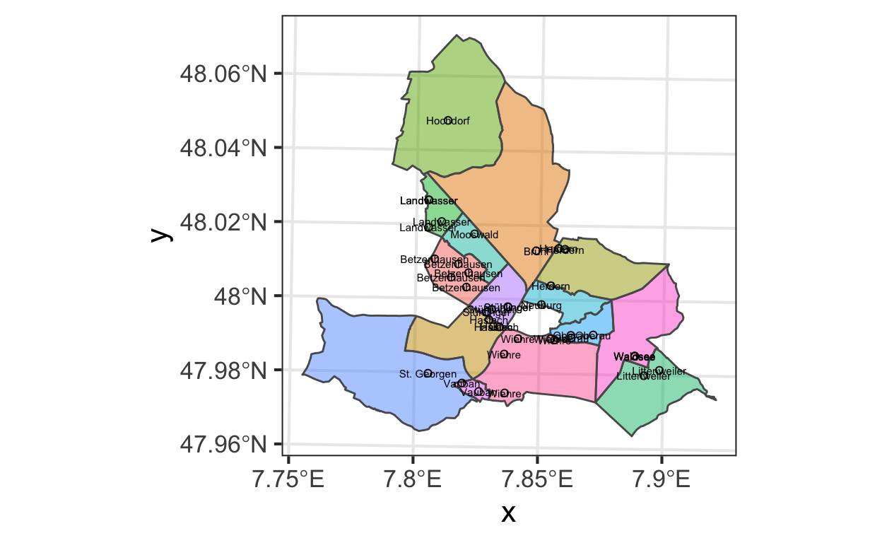
At the end 3 layers are combined to make a map with districts, points for the HOBO locations and the name of the district for each HOBO. To improve the map you can labelöing each district only one time instead multiple times for each HOBO. How?
ggplot() +
    geom_sf(data = hobo_districts, aes(fill = name), alpha = .5)+
    geom_sf(data = hobo_sfd, pch = 21)+
    geom_sf_text(data = hobo_sfd, aes(label = name), size = 2)+
    theme_bw(16)+
    guides(fill = FALSE)
Distances between the HOBOs
dist <- st_distance(hobo_sfd)
dist[1:3,]
Units: [m]
         [,1]     [,2]     [,3]     [,4]     [,5]     [,6]     [,7]
[1,]    0.000 3576.420 4916.272 3832.559 1357.918 3209.025 2690.810
[2,] 3576.420    0.000 2800.832 4182.208 2663.997 3653.002 1558.012
[3,] 4916.272 2800.832    0.000 2794.727 3565.457 2712.321 2318.610
         [,8]     [,9]    [,10]     [,11]    [,12]    [,13]    [,14]
[1,] 4802.174 8184.634 5218.608 3872.9010 4192.686 2174.905 1617.409
[2,] 5577.487 4610.626 1734.026  404.5231 1097.881 1538.049 3254.125
[3,] 3950.620 5078.925 3601.743 3050.2077 3733.891 2990.707 5423.175
        [,15]     [,16]    [,17]    [,18]    [,19]    [,20]     [,21]
[1,] 2752.625 3525.6703 5941.402 2399.296 4730.022 2035.598  563.5999
[2,] 3277.446  541.9984 2489.826 1294.839 1179.096 1874.160 3317.1488
[3,] 2747.878 3342.8164 4159.749 2880.784 2560.753 2947.280 4974.1261
        [,22]     [,23]    [,24]    [,25]     [,26]    [,27]    [,28]
[1,] 2675.631 4562.3342 1975.660 3840.684 3152.5812 4799.564 3236.968
[2,] 3162.443 2136.4454 2475.051 2502.960  437.7744 5582.333 3599.986
[3,] 2720.764  676.0102 2968.642 1143.783 3003.9952 3959.610 2633.112
         [,29]    [,30]    [,31]     [,32]    [,33]    [,34]    [,35]
[1,] 4992.2199 4980.163 2493.464  777.2709 5152.921 1999.740 5941.402
[2,] 2982.2586 6102.932 1300.097 3766.7312 1818.745 1776.251 2489.826
[3,]  195.2624 4595.480 2718.252 4629.7901 3959.406 3052.422 4159.749
        [,36]    [,37]    [,38]    [,39]
[1,] 2682.581 3216.447 4799.564 5459.688
[2,] 1570.880 2387.178 5582.333 6433.769
[3,] 2322.299 1760.543 3959.610 4745.152
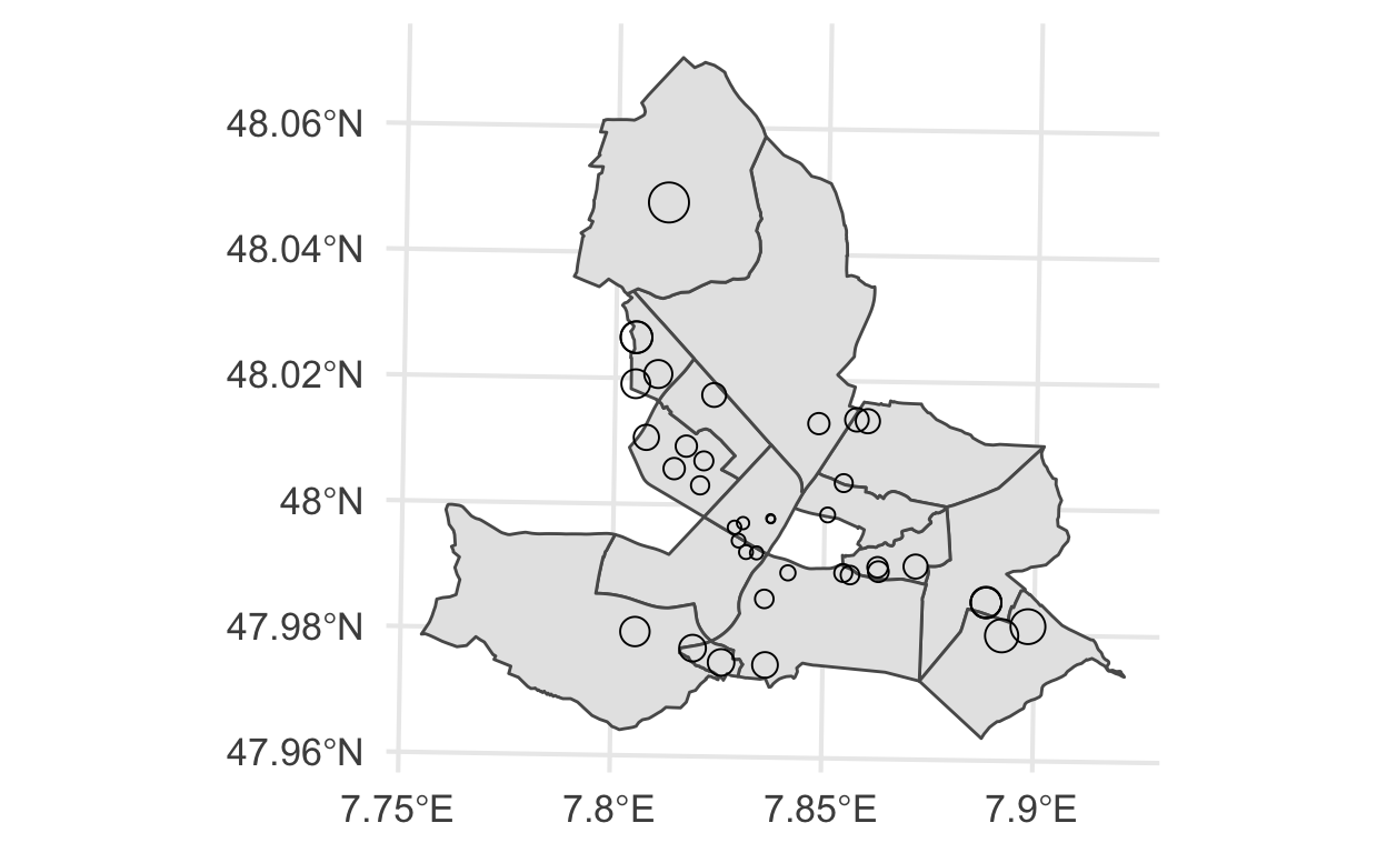
Example: Use the average distance of each HOBO location to all other locations for plotting.
hobo_sfd$mdist <- apply(X = dist, MARGIN = 1, FUN = "mean")

ggplot() +
    geom_sf(data = hobo_districts)+
    geom_sf(data = hobo_sfd, pch = 21, aes(size = mdist))+
    theme_minimal(16)+
    guides(size = FALSE)
Distance between the HOBO locations can be also used as a proxy of similarity. That means if a HOBO is nearer to your location one hypothesis could be that also the temperature indices of this HOBO are more similar compared to those from a HOBO further away.
Interactive maps with leaflet()
Load package library(leaflet).
leaflet(meta) %>%
    addTiles() %>%
    addMarkers(~longitude, ~latitude,
           label = ~as.character(hobo_id))